Newton, The Ultimate: One Weird Trick To Make You A Mathematical Superhero, part 2: Julia, optimization, and automatic differentiation
Because I've heard good things about it, I've switched to the Julia programming language. This post is written as an IJulia notebook. It's like a REPL session, except with text in between, and you can go back and edit and re-run any expression. You can download this notebook and load it up in IJulia to play with the code. This is the first time I'm using Julia, so I very much welcome any tips & corrections.
In part 1 we used Newton's method to solve equations \(f(x) = 0\). Now we're going to use Newton's method for optimization. Optimization in math doesn't mean making something run faster; it means finding the maximum or minimum of a function:
\[\text{minimize } f(x)\]
As you may know, we can find such a minimum or maximum by solving
\[f'(x) = 0\]
We will use Newton's method to find a solution to that equation.
The Tent Company
The company Zelte GmbH makes tents with a circular groundsheet and conical roof. The ground sheet will have radius \(r\) and the roof will have height \(h\):
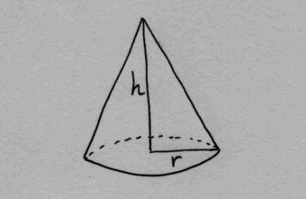
The marketing department wants a tent with a specific volume \(V\), but the purchase management department wants to buy the least amount of tent sheet possible. The question is what is the best shape to minimize the amount of tent sheet?
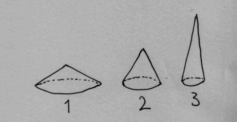
Do we need a wide and short tent? Or a slim and tall? Or something in between?
The volume of the tent and the total area of the tent sheet are given by these equations:
\[\begin{align}V & = \frac{1}{3} \pi r^2 h\\ A & = \pi r^2 + \pi r \sqrt{r^2 + h^2} \end{align}\]
Since the volume is given to us by the marketing department, we rewrite the volume equation as follows:
\[ h = \frac{3V}{\pi r^2} \]
and we plug it into the area equation:
\[ A = \pi r^2 + \pi r \sqrt{r^2 + \left(\frac{3V}{\pi r^2}\right)^2} \]
Here's the problem we want to solve:
\[ \text{minimize}\;\; \pi r^2 + \pi r \sqrt{r^2 + \left(\frac{3V}{\pi r^2}\right)^2} \]
Lets call that function \(A(r)\). Here's that in Julia code:
A(r) = pi*r^2 + pi*r*sqrt(r^2 + ((3V)/(pi*r^2))^2)
To run that code, we also need to define \(V\):
V = 2.43
Lets plot that function to see what it looks like:
using Winston
fplot(A, [0,10])
xlabel("r")
ylabel("A(r)")

You can visually see the \(r\) that gives us the minimum tent sheet area, but we want to know that \(r\) exactly. To do Newton's method we want to solve \(A'(r) = 0\) and Newton's algorithm for that is:
\[ \text{iterate}\;\; r \leftarrow r - \frac{A'(r)}{A''(r)} \]
Compared to Newton's method for solving equations, we've just added an extra ' everywhere to turn it into Newton's method for optimization. We could try to compute the derivatives by hand, but that's tedious, so let's ask Wolfram Alpha for the first derivative and second derivative. Go check out those links.
Whoa, these derivatives are huge! It's a good thing we didn't try that by hand. But now we have to type those derivatives into our code, and even typing them is very tedious.
Approximating derivatives with finite differences
Instead of computing the derivatives exactly, we can approximate them with this formula:
\[f'(x) \approx \frac{f(x+\epsilon) - f(x-\epsilon)}{2\epsilon}\]
where \(\epsilon\) is a very small number. Lets do it in Julia. We define a function deriv(f) that takes a function and returns a new function that is the derivative of that function, using that approximation:
eps = 0.00001
deriv(f) = x -> (f(x+eps) - f(x-eps))/(2*eps)
dA = deriv(A)
ddA = deriv(dA)
We can now run Newton's method:
r = 6.0 # initial guess
rs = [r] # array where we collect all the steps for visualization
for i = 1:20
    r = r - dA(r) / ddA(r)
    push!(rs,r)
end
Here are the steps of the algorithm visualized:
fplot(A,[0,10])
xlabel("r")
ylabel("A(r)")
oplot(rs,Float64[A(r) for r in rs],"b-o")

As you can see it starts at 6, then jumps to 0.00197, and then creeps to the right until it hits 0.936147.
Automatic differentiation
Approximating derivatives with finite differences isn't such a great idea. It's slow and it is very susceptible to rounding errors. Luckily for us there is something called automatic differentiation. It lets us write any function in Julia, and the automatic differentiation library will compute the exact derivative for us (there are automatic differentiation libraries for many other languages as well). That seems like magic; how does automatic differentiation work? That beyond the scope of this post. You can read the Wikipedia page on automatic differentiation if you want to know the details. I'll use a Julia library called HyperDualNumbers that provides tools for automatic differentiation. We use it by creating a special number which is the original number paired up with derivative information. Then we pass that into our function that we want the derivatives of, and the hyper dual number that comes out carries the derivatives with it. For the details read the documentation of HyperDualNumbers.
using HyperDualNumbers
function derivs(f)
    function derivs_f(x)
        hyper_x = hyper(x, 1.0, 1.0, 0.0)
        hyper_y = f(hyper_x)
        (eps1(hyper_y), eps1eps2(hyper_y))
    end
    derivs_f
end
This defines a function derivs(f) that takes a function and returns a new function which will compute the first and second derivatives and return them in a tuple. Here's an example:
derivs_A = derivs(A)
derivs_A(2.3)
This matches the finite difference approximation:
(dA(2.3), ddA(2.3))
Let's try newton's method with automatic differentiation:
r = 6.0 # initial guess
rs = [r] # array where we collect all the steps for visualization
for i = 1:20
    d_A, dd_A = derivs_A(r)
    r = r - d_A / dd_A
    push!(rs,r)
end
Here are the results:
fplot(A,[0,10])
xlabel("r")
ylabel("A(r)")
oplot(rs,Float64[A(r) for r in rs],"b-o")

So what's the shape of the tent?
h = 3V / (pi*r^2)
(r,h)
Here's what it looks like:
p = FramedPlot(aspect_ratio = 1)
add(p,Curve([0,-r,r,0],[h,0,0,h],color="blue"))

That's our tent, I hope Zelte GmbH will be happy.
Conclusion
We've used Newton's algoritm for optimization. There's still some basics to cover:
- Sometimes a Newton step goes way too far. This happens when the function looks linear. We can solve that using a line search: if the step goes too far, we take a smaller step.
- What happens if we have multiple minima or maxima? Then Newton step can go in the wrong direction. To solve that we need a fallback to gradient descent.
After that we can get to the really interesting stuff like machine learning and image denoising :)
I welcome any feedback: is this easy to understand, or hard? Is it going too fast, or too slow? How's the IJulia notebook format?
See you next time!